| Revision as of 16:21, 21 July 2007 editIgny (talk | contribs)Extended confirmed users4,699 editsm →Definition← Previous edit | Revision as of 16:16, 22 July 2007 edit undoOleg Alexandrov (talk | contribs)Administrators47,244 edits rv, you don't need to take a kernel with variance 1Next edit → | ||
| Line 7: | Line 7: | ||
| :<math>\widehat{f}_h(x)=\frac{1}{Nh}\sum_{i=1}^N K\left(\frac{x-x_i}{h}\right)</math> | :<math>\widehat{f}_h(x)=\frac{1}{Nh}\sum_{i=1}^N K\left(\frac{x-x_i}{h}\right)</math> | ||
| where ''K'' is some ] and ''h'' is the bandwidth (] parameter). Quite often ''K'' is taken to be a |
where ''K'' is some ] and ''h'' is the bandwidth (] parameter). Quite often ''K'' is taken to be a ] with ] zero and ] σ<sup>2</sup>: | ||
| :<math>K(x) = {1 \over \sqrt{2\pi} }\,e^{-x^2}.</math> | :<math>K(x) = {1 \over \sigma\sqrt{2\pi} }\,e^{-{x^2 / 2\sigma^2}}.</math> | ||
| ==Intuition== | ==Intuition== | ||
Revision as of 16:16, 22 July 2007

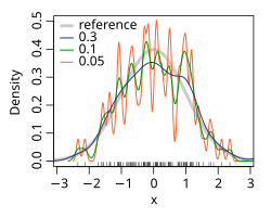
In statistics, the kernel density estimation (or Parzen window method, named after Emanuel Parzen) is a way of estimating the probability density function of a random variable. As an illustration, given some data about a sample of a population, the kernel density estimation makes it possible to extrapolate the data to the entire population.
Definition
If x1, x2, ..., xN ~ f is a IID sample of a random variable, then the kernel density approximation of its probability density function is
where K is some kernel and h is the bandwidth (smoothing parameter). Quite often K is taken to be a Gaussian function with mean zero and variance σ:
Intuition
Although less smooth density estimators such as the histogram density estimator can be made to be asymptotically consistent, others are often either discontinuous or converge at slower rates than the kernel density estimator. Rather than grouping observations together in bins, the kernel density estimator can be thought to place small "bumps" at each observation, determined by the kernel function. The estimator consists of a "sum of bumps" and is clearly smoother as a result (see below image).

Properties
Let be the L risk function for f. Under weak assumptions on f and K,
- where .
By minimizing the theoretical risk function, it can be shown that the optimal bandwidth is
where
When the optimal choice of bandwidth is chosen, the risk function is for some constant c4 > 0. It can be shown that, under weak assumptions, there cannot exist a non-parametric estimator that converges at a faster rate than the kernel estimator. Note that the n rate is slower than the typical n convergence rate of parametric methods.
Statistical implementation
- In Stata, it is implemented through
kdensity; for examplehistogram x, kdensity. - In R, it is implemented through the
densityfunction.
See also
References
- Parzen E. (1962). On estimation of a probability density function and mode, Ann. Math. Stat. 33, pp. 1065-1076.
- Duda, R. and Hart, P. (1973). Pattern Classification and Scene Analysis. John Wiley & Sons. ISBN 0-471-22361-1.
- Wasserman, L. (2005). All of Statistics: A Concise Course in Statistical Inference, Springer Texts in Statistics.
External links
- Introduction to kernel density estimation
- Free Online Software (Calculator) computes the Kernel Density Estimation for any data series according to the following Kernels: Gaussian, Epanechnikov, Rectangular, Triangular, Biweight, Cosine, and Optcosine.


 be the L
  where
where  .
.


 for some constant c4 > 0. It can be shown that, under weak assumptions, there cannot exist a non-parametric estimator that converges at a faster rate than the kernel estimator. Note that the n rate is slower than the typical n convergence rate of parametric methods.