| Revision as of 03:36, 14 November 2016 editNovarank (talk | contribs)14 editsm →Applications: minor fixes.Tag: Visual edit← Previous edit | Revision as of 21:03, 14 November 2016 edit undo129.55.200.20 (talk) →Mathematical RepresentationNext edit → | ||
| Line 3: | Line 3: | ||
| == Mathematical Representation == | == Mathematical Representation == | ||
| ] | ] | ||
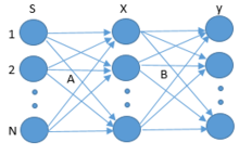
| The following equation is problem, the individual source signals, s(t), is mixed by coefficients, A, that produces mixed signals, x(t). | The following equation is the problem, the individual source signals, s(t), is mixed by coefficients, A, that produces mixed signals, x(t). | ||
| <math>x(t) = A*s(t)</math> | <math>x(t) = A*s(t)</math> | ||
Revision as of 21:03, 14 November 2016
Blind signal separation (BSS), also known as blind source separation, is the separation of a set of source signals from a set of mixed signals, without the aid of information (or with very little information) about the source signals or the mixing process. This problem is in general highly underdetermined, but useful solutions can be derived under a surprising variety of conditions. Much of the early literature in this field focuses on the separation of temporal signals such as audio. However, blind signal separation is now routinely performed on multidimensional data, such as images and tensors, which may involve no time dimension whatsoever.
Mathematical Representation

The following equation is the problem, the individual source signals, s(t), is mixed by coefficients, A, that produces mixed signals, x(t).
The following equation BSS separates the mixed signals, x(t) by finding and using coefficients, B, to separate and get approximation of original signal, y(t).
Applications
At cocktail party, there a group of people talking at same time. You have multiple microphones that picking up mixed signals but you want to only hear of one person talking. BSS can be used to separate the individual sources by using mixed signals.

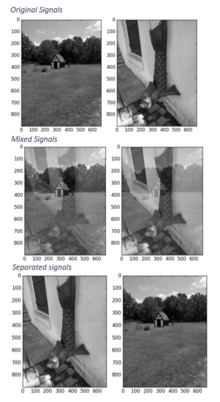
In Figure 2, it shows the the basic concept of BSS. The individual source signals are shown as well as the mixed signals which are received signals. BSS is used to separate the mixed signals with only knowing mixed signals and nothing about original signal or how they were mixed. The separated signals are only approximations of the source signals. The separated images, were separated using Python and the Shogun toolbox using Joint Approximation Diagonalization of Eigen-matrices (JADE) algorithm which is based off ICA. This process was done following the tutorial. This toolbox method can be used with multi-dimensions but for an easy visual aspect images(2-D) were used.
Real world applications
- Brain Imaging
- Stock Prediction
- Seismic Monitoring
- Text Document Analysis
Approaches
Since the chief difficulty of the problem is its underdetermination, methods for blind source separation generally seek to narrow the set of possible solutions in a way that is unlikely to exclude the desired solution. In one approach, exemplified by principal and independent component analysis, one seeks source signals that are minimally correlated or maximally independent in a probabilistic or information-theoretic sense. A second approach, exemplified by nonnegative matrix factorization, is to impose structural constraints on the source signals. These structural constraints may be derived from a generative model of the signal, but are more commonly heuristics justified by good empirical performance. A common theme in the second approach is to impose some kind of low-complexity constraint on the signal, such as sparsity in some basis for the signal space. This approach can be particularly effective if one requires not the whole signal, but merely its most salient features.
Methods
There are different methods of blind signal separation:
- Principal components analysis
- Singular value decomposition
- Independent component analysis
- Dependent component analysis
- Non-negative matrix factorization
- Low-complexity coding and decoding
- Stationary subspace analysis
- Common spatial pattern
See also
References
- Jean-Francois Cardoso “Blind Signal Separation: statistical Principles” http://citeseerx.ist.psu.edu/viewdoc/download?doi=10.1.1.462.9738&rep=rep1&type=pdf
- ^ Aapo Hyvarinen, Juha Karhunen, and Erkki Oja. “Independent Component Analysis” https://www.cs.helsinki.fi/u/ahyvarin/papers/bookfinal_ICA.pdf pp147 – 148, pp 407, pp 441-442, pp 448
- Kevin Hughes “Blind Source Separation on Images with Shogun” http://shogun-toolbox.org/static/notebook/current/bss_image.html
- Ranjan Acharyya (editors) (2008): A New Approach for Blind Source Separation of Convolutive Sources, ISBN 3-639-07797-0 ISBN 978-3639077971
External links
- Blind source separation flash presentation
- Removing electroencephalographic artifacts by blind source separation
This signal processing-related article is a stub. You can help Misplaced Pages by expanding it. |

