In statistics, single-linkage clustering is one of several methods of hierarchical clustering. It is based on grouping clusters in bottom-up fashion (agglomerative clustering), at each step combining two clusters that contain the closest pair of elements not yet belonging to the same cluster as each other.
This method tends to produce long thin clusters in which nearby elements of the same cluster have small distances, but elements at opposite ends of a cluster may be much farther from each other than two elements of other clusters. For some classes of data, this may lead to difficulties in defining classes that could usefully subdivide the data. However, it is popular in astronomy for analyzing galaxy clusters, which may often involve long strings of matter; in this application, it is also known as the friends-of-friends algorithm.
Overview of agglomerative clustering methods
In the beginning of the agglomerative clustering process, each element is in a cluster of its own. The clusters are then sequentially combined into larger clusters, until all elements end up being in the same cluster. At each step, the two clusters separated by the shortest distance are combined. The function used to determine the distance between two clusters, known as the linkage function, is what differentiates the agglomerative clustering methods.
In single-linkage clustering, the distance between two clusters is determined by a single pair of elements: those two elements (one in each cluster) that are closest to each other. The shortest of these pairwise distances that remain at any step causes the two clusters whose elements are involved to be merged. The method is also known as nearest neighbour clustering. The result of the clustering can be visualized as a dendrogram, which shows the sequence in which clusters were merged and the distance at which each merge took place.
Mathematically, the linkage function – the distance D(X,Y) between clusters X and Y – is described by the expression
where X and Y are any two sets of elements considered as clusters, and d(x,y) denotes the distance between the two elements x and y.
Naive algorithm
The following algorithm is an agglomerative scheme that erases rows and columns in a proximity matrix as old clusters are merged into new ones. The proximity matrix contains all distances . The clusterings are assigned sequence numbers and is the level of the -th clustering. A cluster with sequence number m is denoted (m) and the proximity between clusters and is denoted .
The single linkage algorithm is composed of the following steps:
- Begin with the disjoint clustering having level and sequence number .
- Find the most similar pair of clusters in the current clustering, say pair , according to where the minimum is over all pairs of clusters in the current clustering.
- Increment the sequence number: . Merge clusters and into a single cluster to form the next clustering . Set the level of this clustering to
- Update the proximity matrix, , by deleting the rows and columns corresponding to clusters and and adding a row and column corresponding to the newly formed cluster. The proximity between the new cluster, denoted and an old cluster is defined as .
- If all objects are in one cluster, stop. Else, go to step 2.
Working example
This working example is based on a JC69 genetic distance matrix computed from the 5S ribosomal RNA sequence alignment of five bacteria: Bacillus subtilis (), Bacillus stearothermophilus (), Lactobacillus viridescens (), Acholeplasma modicum (), and Micrococcus luteus ().
First step
- First clustering
Let us assume that we have five elements and the following matrix of pairwise distances between them:
| a | b | c | d | e | |
|---|---|---|---|---|---|
| a | 0 | 17 | 21 | 31 | 23 |
| b | 17 | 0 | 30 | 34 | 21 |
| c | 21 | 30 | 0 | 28 | 39 |
| d | 31 | 34 | 28 | 0 | 43 |
| e | 23 | 21 | 39 | 43 | 0 |
In this example, is the lowest value of , so we cluster elements a and b.
- First branch length estimation
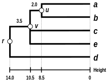
Let u denote the node to which a and b are now connected. Setting ensures that elements a and b are equidistant from u. This corresponds to the expectation of the ultrametricity hypothesis. The branches joining a and b to u then have lengths (see the final dendrogram)
- First distance matrix update
We then proceed to update the initial proximity matrix into a new proximity matrix (see below), reduced in size by one row and one column because of the clustering of a with b. Bold values in correspond to the new distances, calculated by retaining the minimum distance between each element of the first cluster and each of the remaining elements:
Italicized values in are not affected by the matrix update as they correspond to distances between elements not involved in the first cluster.
Second step
- Second clustering
We now reiterate the three previous actions, starting from the new distance matrix :
| (a,b) | c | d | e | |
|---|---|---|---|---|
| (a,b) | 0 | 21 | 31 | 21 |
| c | 21 | 0 | 28 | 39 |
| d | 31 | 28 | 0 | 43 |
| e | 21 | 39 | 43 | 0 |
Here, and are the lowest values of , so we join cluster with element c and with element e.
- Second branch length estimation
Let v denote the node to which , c and e are now connected. Because of the ultrametricity constraint, the branches joining a or b to v, and c to v, and also e to v are equal and have the following total length:
We deduce the missing branch length:
- Second distance matrix update
We then proceed to update the matrix into a new distance matrix (see below), reduced in size by two rows and two columns because of the clustering of with c and with e :
Final step
The final matrix is:
| ((a,b),c,e) | d | |
|---|---|---|
| ((a,b),c,e) | 0 | 28 |
| d | 28 | 0 |
So we join clusters and .
Let denote the (root) node to which and are now connected. The branches joining and to then have lengths:
We deduce the remaining branch length:
The single-linkage dendrogram

The dendrogram is now complete. It is ultrametric because all tips (, , , , and ) are equidistant from :
The dendrogram is therefore rooted by , its deepest node.
Other linkages
The naive algorithm for single linkage clustering is essentially the same as Kruskal's algorithm for minimum spanning trees. However, in single linkage clustering, the order in which clusters are formed is important, while for minimum spanning trees what matters is the set of pairs of points that form distances chosen by the algorithm.
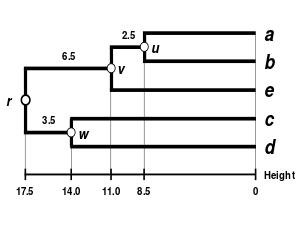
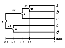
Alternative linkage schemes include complete linkage clustering, average linkage clustering (UPGMA and WPGMA), and Ward's method. In the naive algorithm for agglomerative clustering, implementing a different linkage scheme may be accomplished simply by using a different formula to calculate inter-cluster distances in the algorithm. The formula that should be adjusted has been highlighted using bold text in the above algorithm description. However, more efficient algorithms such as the one described below do not generalize to all linkage schemes in the same way.
 |

|
 |
 |
| Single-linkage clustering | Complete-linkage clustering | Average linkage clustering: WPGMA | Average linkage clustering: UPGMA |
Faster algorithms
The naive algorithm for single-linkage clustering is easy to understand but slow, with time complexity . In 1973, R. Sibson proposed an algorithm with time complexity and space complexity (both optimal) known as SLINK. The slink algorithm represents a clustering on a set of numbered items by two functions. These functions are both determined by finding the smallest cluster that contains both item and at least one larger-numbered item. The first function, , maps item to the largest-numbered item in cluster . The second function, , maps item to the distance associated with the creation of cluster . Storing these functions in two arrays that map each item number to its function value takes space , and this information is sufficient to determine the clustering itself. As Sibson shows, when a new item is added to the set of items, the updated functions representing the new single-linkage clustering for the augmented set, represented in the same way, can be constructed from the old clustering in time . The SLINK algorithm then loops over the items, one by one, adding them to the representation of the clustering.
An alternative algorithm, running in the same optimal time and space bounds, is based on the equivalence between the naive algorithm and Kruskal's algorithm for minimum spanning trees. Instead of using Kruskal's algorithm, one can use Prim's algorithm, in a variation without binary heaps that takes time and space to construct the minimum spanning tree (but not the clustering) of the given items and distances. Then, applying Kruskal's algorithm to the sparse graph formed by the edges of the minimum spanning tree produces the clustering itself in an additional time and space .
See also
- Cluster analysis
- Complete-linkage clustering
- Hierarchical clustering
- Molecular clock
- Neighbor-joining
- UPGMA
- WPGMA
References
- Everitt B (2011). Cluster analysis. Chichester, West Sussex, U.K: Wiley. ISBN 9780470749913.
- Feigelson, Eric (2012). "Classification in astronomy: past and present". In Way, Michael J.; Scargle, Jeffrey D.; Ali, Kamal M.; Srivastava, Ashok N. (eds.). Advances in Machine Learning and Data Mining for Astronomy. Chapman and Hall/CRC. pp. 3–10. Bibcode:2012amld.book....3F. doi:10.1201/b11822-7 (inactive 2024-11-12).
{{cite book}}: CS1 maint: DOI inactive as of November 2024 (link) - Legendre P, Legendre L (1998). Numerical Ecology. Developments in Environmental Modelling. Vol. 20 (Second English ed.). Amsterdam: Elsevier.
- Erdmann VA, Wolters J (1986). "Collection of published 5S, 5.8S and 4.5S ribosomal RNA sequences". Nucleic Acids Research. 14 Suppl (Suppl): r1-59. doi:10.1093/nar/14.suppl.r1. PMC 341310. PMID 2422630.
- Olsen GJ (1988). "Phylogenetic analysis using ribosomal RNA". In Noller HF Jr, Moldave K (eds.). Ribosomes. Methods in Enzymology. Vol. 164. pp. 793–812. doi:10.1016/s0076-6879(88)64084-5. ISBN 978-0-12-182065-7. PMID 3241556.
- Murtagh F, Contreras P (2012). "Algorithms for hierarchical clustering: an overview". Wiley Interdisciplinary Reviews: Data Mining and Knowledge Discovery. 2 (1). Wiley Online Library: 86–97. doi:10.1002/widm.53.
- Sibson R (1973). "SLINK: an optimally efficient algorithm for the single-link cluster method" (PDF). The Computer Journal. 16 (1). British Computer Society: 30–34. doi:10.1093/comjnl/16.1.30.
- Gan G (2007). Data clustering : theory, algorithms, and applications. Philadelphia, Pa. Alexandria, Va: SIAM, Society for Industrial and Applied Mathematics American Statistical Association. ISBN 9780898716238.
- Gower JC, Ross GJ (1969). "Minimum spanning trees and single linkage cluster analysis". Journal of the Royal Statistical Society, Series C. 18 (1): 54–64. doi:10.2307/2346439. JSTOR 2346439. MR 0242315..

 proximity matrix
  contains all distances
  . The clusterings are assigned sequence numbers
  and
and  is the level of the
  -th clustering. A cluster with sequence number m is denoted (m) and the proximity between clusters
  and
and  is denoted
  .
.
 and sequence number
  .
. , according to
  where the minimum is over all pairs of clusters in the current clustering.
 . Merge clusters
  . Set the level of this clustering to
 and an old cluster
  is defined as
  .
. ),
),  ),
),  ),
),  ), and
  ).
).
 and the following matrix
  of pairwise distances between them:
 is the lowest value of
  ensures that elements a and b are equidistant from u. This corresponds to the expectation of the
  (
( (see below), reduced in size by one row and one column because of the clustering of a with b.
Bold values in
  and each of the remaining elements:

 and
and  are the lowest values of
 (
( (see below), reduced in size by two rows and two columns because of the clustering of
 and
and  denote the (root) node to which


 . In 1973, R. Sibson proposed an algorithm with time complexity
  and space complexity
  (both optimal) known as SLINK. The slink algorithm represents a clustering on a set of
  numbered items by two functions. These functions are both determined by finding the smallest cluster
  that contains both item
  and at least one larger-numbered item.
The first function,
  , maps item
  , maps item
  and space