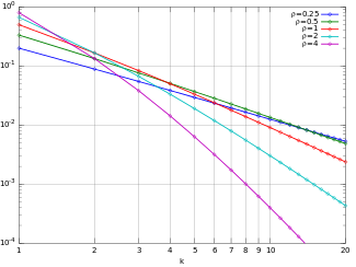
Probability mass function Yule–Simon PMF on a log-log scale. (Note that the function is only defined at integer values of k. The connecting lines do not indicate continuity.) | |||
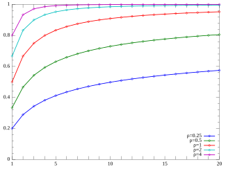
Cumulative distribution function Yule–Simon CMF. (Note that the function is only defined at integer values of k. The connecting lines do not indicate continuity.) | |||
| Parameters | shape (real) | ||
|---|---|---|---|
| Support | |||
| PMF | |||
| CDF | |||
| Mean | for | ||
| Mode | |||
| Variance | for | ||
| Skewness | for | ||
| Excess kurtosis | for | ||
| MGF | does not exist | ||
| CF | |||
In probability and statistics, the Yule–Simon distribution is a discrete probability distribution named after Udny Yule and Herbert A. Simon. Simon originally called it the Yule distribution.
The probability mass function (pmf) of the Yule–Simon (ρ) distribution is
for integer and real , where is the beta function. Equivalently the pmf can be written in terms of the rising factorial as
where is the gamma function. Thus, if is an integer,
The parameter can be estimated using a fixed point algorithm.
The probability mass function f has the property that for sufficiently large k we have

This means that the tail of the Yule–Simon distribution is a realization of Zipf's law: can be used to model, for example, the relative frequency of the th most frequent word in a large collection of text, which according to Zipf's law is inversely proportional to a (typically small) power of .
Occurrence
The Yule–Simon distribution arose originally as the limiting distribution of a particular model studied by Udny Yule in 1925 to analyze the growth in the number of species per genus in some higher taxa of biotic organisms. The Yule model makes use of two related Yule processes, where a Yule process is defined as a continuous time birth process which starts with one or more individuals. Yule proved that when time goes to infinity, the limit distribution of the number of species in a genus selected uniformly at random has a specific form and exhibits a power-law behavior in its tail. Thirty years later, the Nobel laureate Herbert A. Simon proposed a time-discrete preferential attachment model to describe the appearance of new words in a large piece of a text. Interestingly enough, the limit distribution of the number of occurrences of each word, when the number of words diverges, coincides with that of the number of species belonging to the randomly chosen genus in the Yule model, for a specific choice of the parameters. This fact explains the designation Yule–Simon distribution that is commonly assigned to that limit distribution. In the context of random graphs, the Barabási–Albert model also exhibits an asymptotic degree distribution that equals the Yule–Simon distribution in correspondence of a specific choice of the parameters and still presents power-law characteristics for more general choices of the parameters. The same happens also for other preferential attachment random graph models.
The preferential attachment process can also be studied as an urn process in which balls are added to a growing number of urns, each ball being allocated to an urn with probability linear in the number (of balls) the urn already contains.
The distribution also arises as a compound distribution, in which the parameter of a geometric distribution is treated as a function of random variable having an exponential distribution. Specifically, assume that follows an exponential distribution with scale or rate :
with density
Then a Yule–Simon distributed variable K has the following geometric distribution conditional on W:
The pmf of a geometric distribution is
for . The Yule–Simon pmf is then the following exponential-geometric compound distribution:
The maximum likelihood estimator for the parameter given the observations is the solution to the fixed point equation
where are the rate and shape parameters of the gamma distribution prior on .
This algorithm is derived by Garcia by directly optimizing the likelihood. Roberts and Roberts
generalize the algorithm to Bayesian settings with the compound geometric formulation described above. Additionally, Roberts and Roberts are able to use the Expectation Maximisation (EM) framework to show convergence of the fixed point algorithm. Moreover, Roberts and Roberts derive the sub-linearity of the convergence rate for the fixed point algorithm. Additionally, they use the EM formulation to give 2 alternate derivations of the standard error of the estimator from the fixed point equation. The variance of the estimator is
the standard error is the square root of the quantity of this estimate divided by N.
Generalizations
The two-parameter generalization of the original Yule distribution replaces the beta function with an incomplete beta function. The probability mass function of the generalized Yule–Simon(ρ, α) distribution is defined as
with . For the ordinary Yule–Simon(ρ) distribution is obtained as a special case. The use of the incomplete beta function has the effect of introducing an exponential cutoff in the upper tail.
See also
Bibliography
- Colin Rose and Murray D. Smith, Mathematical Statistics with Mathematica. New York: Springer, 2002, ISBN 0-387-95234-9. (See page 107, where it is called the "Yule distribution".)
References
- Simon, H. A. (1955). "On a class of skew distribution functions". Biometrika. 42 (3–4): 425–440. doi:10.1093/biomet/42.3-4.425.
- ^ Garcia Garcia, Juan Manuel (2011). "A fixed-point algorithm to estimate the Yule-Simon distribution parameter". Applied Mathematics and Computation. 217 (21): 8560–8566. doi:10.1016/j.amc.2011.03.092.
- Yule, G. U. (1924). "A Mathematical Theory of Evolution, based on the Conclusions of Dr. J. C. Willis, F.R.S". Philosophical Transactions of the Royal Society B. 213 (402–410): 21–87. doi:10.1098/rstb.1925.0002.
- Pachon, Angelica; Polito, Federico; Sacerdote, Laura (2015). "Random Graphs Associated to Some Discrete and Continuous Time Preferential Attachment Models". Journal of Statistical Physics. 162 (6): 1608–1638. arXiv:1503.06150. doi:10.1007/s10955-016-1462-7. S2CID 119168040.
- ^ Roberts, Lucas; Roberts, Denisa (2017). "An Expectation Maximization Framework for Preferential Attachment Models". arXiv:1710.08511 .
 shape (


 for
for 

 for
for 
 for
for 
 for
for 


 and
and  , where
  is the
 is the
  is an integer,


 can be used to model, for example, the relative frequency of the
  th most frequent word in a large collection of text, which according to Zipf's law is
  follows an exponential distribution with
  or rate


 is the solution to the fixed point equation

 are the rate and shape parameters of the
  estimator is


 . For
. For  the ordinary Yule–Simon(ρ) distribution is obtained as a special case. The use of the incomplete beta function has the effect of introducing an exponential cutoff in the upper tail.